Tutorial: skpro Interface

Probabilistic Regression with Full Predictive Distributions

The partition_tree.skpro module provides probabilistic regressors that return full predictive distributions instead of point estimates. They extend skpro’s BaseProbaRegressor, giving you access to PDF, CDF, quantiles (PPF), sampling, and more.

For a worked example with a lattice-valued response, see Quantized Targets.

Available Estimators

Class	Description
PartitionTreeRegressor	Single probabilistic tree
PartitionForestRegressor	Ensemble of probabilistic trees (density averaging)

Both return an IntervalDistribution from predict_proba — a piecewise-constant distribution defined over disjoint intervals.

---

1. Basic Usage

1.1 Fit and Predict

import pandas as pd
from sklearn.datasets import fetch_california_housing
from sklearn.model_selection import train_test_split

from partition_tree.skpro import PartitionTreeRegressor

# Load data as DataFrames (skpro estimators work best with pandas)
housing = fetch_california_housing(as_frame=True)
X = housing.data
y = housing.target.rename("MedHouseVal").to_frame()

X_train, X_test, y_train, y_test = train_test_split(
    X, y, test_size=0.2, random_state=42
)

# Fit
pt = PartitionTreeRegressor(
    max_leaves=200,
    min_samples_x=100,
    min_samples_y=100,
    random_state=42,
)
pt.fit(X_train, y_train)

# Point predictions (posterior mean over the piecewise density)
y_pred = pt.predict(X_test)
print(y_pred.head())

       MedHouseVal
20046     0.934039
3024      0.927517
15663     3.820700
20484     2.259561
9814      2.363631

1.2 Probabilistic Predictions

predict_proba returns an IntervalDistribution object:

dist = pt.predict_proba(X_test)
print(type(dist))
# <class 'partition_tree.skpro.distribution.IntervalDistribution'>

<class 'partition_tree.skpro.distribution.IntervalDistribution'>

From this distribution you can extract:

# Posterior mean
mean = dist.mean()

# Posterior variance
var = dist.var()

# Quantiles via the percent-point function (inverse CDF)
median   = dist.ppf(0.5)
lower_90 = dist.ppf(0.05)
upper_90 = dist.ppf(0.95)

# Random samples
samples = dist.sample(n_samples=100)

# PDF / CDF evaluated at specific points
pdf_vals = dist.pdf(y_test)
cdf_vals = dist.cdf(y_test)

---

2. Prediction Intervals

One of the key advantages of probabilistic predictions is the ability to construct prediction intervals at any confidence level.

import numpy as np

# 80% prediction interval: [10th percentile, 90th percentile]
lower_80 = dist.ppf(0.10)["MedHouseVal"]
upper_80 = dist.ppf(0.90)["MedHouseVal"]

# Check empirical coverage
y_true = y_test.values
covered = ((y_true >= lower_80.values) & (y_true <= upper_80.values)).mean()
print(f"80% PI coverage: {covered:.1%}")

80% PI coverage: 43.6%

---

3. Visualizing the Predictive PDF

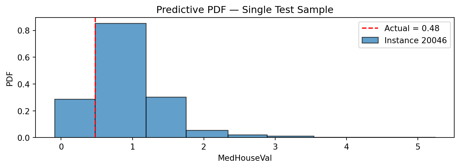
The IntervalDistribution has a built-in plot method that draws the piecewise-constant density as histogram-like bars:

import matplotlib.pyplot as plt

# Plot the predictive PDF for a single test sample
idx = y_test.index[0]
dist_single = dist.loc[idx]

fig, ax = plt.subplots(figsize=(8, 3))
dist_single.plot(ax=ax, alpha=0.7)
ax.axvline(
    y_test.loc[idx].item(),
    color="red",
    linestyle="--",
    label=f"Actual = {y_test.loc[idx].item():.2f}",
)
ax.set_xlabel("MedHouseVal")
ax.set_ylabel("PDF")
ax.set_title("Predictive PDF — Single Test Sample")
ax.legend()
plt.tight_layout()
plt.show()

Multiple samples side by side

fig, axes = plt.subplots(1, 4, figsize=(16, 3))
for ax, i in zip(axes, range(4)):
    row_idx = y_test.index[i]
    dist_single = dist.loc[row_idx]
    dist_single.plot(ax=ax, alpha=0.7)
    ax.axvline(y_test.iloc[i].item(), color="red", linestyle="--", linewidth=1.5)
    ax.set_title(f"Sample {i}")
    ax.set_xlabel("y")

plt.suptitle("Predictive PDFs — PartitionTreeRegressor", y=1.02)
plt.tight_layout()
plt.show()

---

4. Partition Forest (Ensemble)

PartitionForestRegressor averages the conditional densities from multiple trees, producing smoother and better-calibrated distributions.

from partition_tree.skpro import PartitionForestRegressor

pf = PartitionForestRegressor(
    n_estimators=50,
    random_state=42,
    min_samples_x=100,
    min_samples_y=100,
    output_distribution="merged",
)
pf.fit(X_train, y_train)

dist_forest = pf.predict_proba(X_test)
y_pred_forest = pf.predict(X_test)

Comparing Tree vs Forest

from sklearn.metrics import mean_absolute_error, r2_score

y_mean_tree   = pt.predict(X_test)["MedHouseVal"]
y_mean_forest = pf.predict(X_test)["MedHouseVal"]

# Point-estimate metrics
results = pd.DataFrame({
    "Model": ["PartitionTree", "PartitionForest"],
    "MAE": [
        mean_absolute_error(y_test, y_mean_tree),
        mean_absolute_error(y_test, y_mean_forest),
    ],
    "R²": [
        r2_score(y_test, y_mean_tree),
        r2_score(y_test, y_mean_forest),
    ],
})
print(results.to_string(index=False))

Coverage comparison

lower_f = dist_forest.ppf(0.10)["MedHouseVal"]
upper_f = dist_forest.ppf(0.90)["MedHouseVal"]
covered_f = ((y_true >= lower_f.values) & (y_true <= upper_f.values)).mean()

print(f"Tree   80% PI coverage: {covered:.1%}")
print(f"Forest 80% PI coverage: {covered_f:.1%}")

---

5. Per-Tree Distributions

The forest exposes predict_proba_per_tree to access each individual tree’s distribution before mixing:

per_tree_dists = pf.predict_proba_per_tree(X_test)

print(f"Number of trees: {len(per_tree_dists)}")
print(f"Type: {type(per_tree_dists[0])}")

# Compare posterior means across trees
tree_means = np.array([d.mean().values.ravel() for d in per_tree_dists])
print(f"Mean std across trees: {tree_means.std(axis=0).mean():.4f}")

---

6. Feature Importances

The tree exposes feature importances based on the log-loss gain accumulated across all splits:

importances = pt.get_feature_importances(normalize=True)
for feat, imp in importances.items():
    print(f"  {feat:>20s}: {imp:.4f}")

---

7. Leaf Information

Inspect the partition structure:

leaves = pt.get_leaves_info()
print(f"Number of leaves: {len(leaves)}")
print(f"Keys per leaf: {list(leaves[0].keys())}")

---

8. Full IntervalDistribution API

The IntervalDistribution object returned by predict_proba supports:

Method	Returns
mean()	Posterior mean — pd.DataFrame
var()	Posterior variance — pd.DataFrame
pdf(x)	Density at x — pd.DataFrame
log_pdf(x)	Log-density at x — pd.DataFrame
cdf(x)	CDF at x — pd.DataFrame
ppf(q)	Quantile at level q — pd.DataFrame
sample(n_samples)	Random samples — pd.DataFrame
energy(x)	Energy score — pd.DataFrame
plot(ax)	Plot the piecewise-constant PDF

All outputs are pandas DataFrames indexed consistently with the input.

---

9. Tips

TipUse pandas DataFrames

The skpro estimators work best when X and y are pandas DataFrames / Series. Column names are preserved through the pipeline and appear in feature importances.

TipForest for better calibration

If your 80% prediction intervals have coverage far from 80%, try using PartitionForestRegressor — density averaging typically improves calibration.

TipScaling features

Although tree-based methods are invariant to monotone feature transformations, scaling can help when feature magnitudes differ wildly, since the split search evaluates thresholds in the original feature scale.