Tutorial: Probabilistic Regression

Full predictive distributions with the skpro interface

The partition_tree.skpro module exposes the same Partition Tree algorithm through the skpro BaseProbaRegressor interface. Instead of a scalar prediction, predict_proba returns an IntervalDistribution — a piecewise-constant density that you can query for PDF values, CDFs, quantiles, prediction intervals, and random samples.

Just want point predictions?

See the Regression tutorial, which uses the lighter-weight partition_tree.sklearn interface and returns plain NumPy arrays.

Setup

import pandas as pd
from sklearn.datasets import fetch_california_housing
from sklearn.model_selection import train_test_split

housing = fetch_california_housing(as_frame=True)
X = housing.data
y = housing.target.rename("MedHouseVal")

X_train, X_test, y_train, y_test = train_test_split(
    X, y, test_size=0.2, random_state=42
)

1. Baseline — Decision Tree (CART)

CART produces only point predictions, so we use MAE and R² as the comparison baseline.

from sklearn.tree import DecisionTreeRegressor
from sklearn.metrics import root_mean_squared_error, r2_score
import numpy as np


cart = DecisionTreeRegressor(random_state=42)
cart.fit(X_train, y_train)
y_pred_cart = cart.predict(X_test)

print("=== DecisionTreeRegressor (CART) ===")
print(f"RMSE : {root_mean_squared_error(y_test, y_pred_cart):.4f}")
print(f"R²  : {r2_score(y_test, y_pred_cart):.4f}")
print("(no probabilistic output available)")

=== DecisionTreeRegressor (CART) ===
RMSE : 0.7037
R²  : 0.6221
(no probabilistic output available)

2. Single Partition Tree

Fit and point prediction

from partition_tree.skpro import PartitionTreeRegressor

pt = PartitionTreeRegressor(
    min_volume_fraction=0.1,
)
pt.fit(X_train, y_train)

# Point prediction — posterior mean of the conditional density
y_pred_pt = pt.predict(X_test)

print("=== PartitionTreeRegressor ===")
print(f"RMSE : {root_mean_squared_error(y_test, y_pred_pt):.4f}")
print(f"R²  : {r2_score(y_test, y_pred_pt):.4f}")

=== PartitionTreeRegressor ===
RMSE : 0.5879
R²  : 0.7362

Comparison with CART

pd.DataFrame({
    "Model": ["DecisionTree (CART)", "PartitionTree"],
    "RMSE": [
        root_mean_squared_error(y_test, y_pred_cart),
        root_mean_squared_error(y_test, y_pred_pt),
    ],
    "R²": [
        r2_score(y_test, y_pred_cart),
        r2_score(y_test, y_pred_pt),
    ],
}).round(4)

	Model	RMSE	R²
0	DecisionTree (CART)	0.7037	0.6221
1	PartitionTree	0.5879	0.7362

Probabilistic prediction

predict_proba returns an IntervalDistribution:

dist = pt.predict_proba(X_test)
print(type(dist))

<class 'partition_tree.skpro.distribution.IntervalDistribution'>

3. The `IntervalDistribution` API

From the distribution object you can extract:

# Posterior mean (same as predict)
mean = dist.mean()

# Posterior variance
var = dist.var()

# Quantiles via the inverse CDF (percent-point function)
median   = dist.ppf(0.5)
lower_90 = dist.ppf(0.05)
upper_90 = dist.ppf(0.95)

# Random samples from the predictive distribution
samples = dist.sample(n_samples=100)

# PDF / CDF evaluated at specific points
pdf_vals = dist.pdf(y_test.to_frame())
cdf_vals = dist.cdf(y_test.to_frame())

print("mean shape :", mean.shape)
print("var  shape :", var.shape)
print("ppf  shape :", median.shape)

mean shape : (4128, 1)
var  shape : (4128, 1)
ppf  shape : (4128, 1)

Method	Returns
`mean()`	Posterior mean — `pd.DataFrame`
`var()`	Posterior variance — `pd.DataFrame`
`pdf(x)`	Density at `x` — `pd.DataFrame`
`log_pdf(x)`	Log-density at `x` — `pd.DataFrame`
`cdf(x)`	CDF at `x` — `pd.DataFrame`
`ppf(q)`	Quantile at level `q` — `pd.DataFrame`
`sample(n_samples)`	Random samples — `pd.DataFrame`
`energy(x)`	Energy score — `pd.DataFrame`
`plot(ax)`	Plot the piecewise-constant PDF

4. Prediction Intervals

Prediction intervals are constructed directly from the inverse CDF.

import numpy as np

# 80 % prediction interval: [10th percentile, 90th percentile]
lower_80 = dist.ppf(0.10)["MedHouseVal"]
upper_80 = dist.ppf(0.90)["MedHouseVal"]

y_true = y_test.values
covered = ((y_true >= lower_80.values) & (y_true <= upper_80.values)).mean()
print(f"80% PI empirical coverage: {covered:.1%}")

80% PI empirical coverage: 76.1%

Why coverage may differ from the nominal level

The Partition Tree density is learned from training data, so calibration improves with more data and better-tuned hyperparameters. Using PartitionForestRegressor (Section 5) typically yields better-calibrated intervals through density averaging.

5. Visualizing the Predictive PDF

IntervalDistribution has a built-in plot method that renders the piecewise-constant density as histogram-like bars.

import matplotlib.pyplot as plt

# Single test sample
idx = y_test.index[0]
dist_single = dist.loc[[idx]]

fig, ax = plt.subplots(figsize=(8, 3))
dist_single.plot(ax=ax, alpha=0.7)
ax.axvline(
    y_test.loc[idx],
    color="red",
    linestyle="--",
    label=f"Actual = {y_test.loc[idx]:.2f}",
)
ax.set_xlabel("MedHouseVal (×$100k)")
ax.set_ylabel("PDF")
ax.set_title("Predictive PDF — Single Test Sample")
ax.legend()
plt.tight_layout()
plt.show()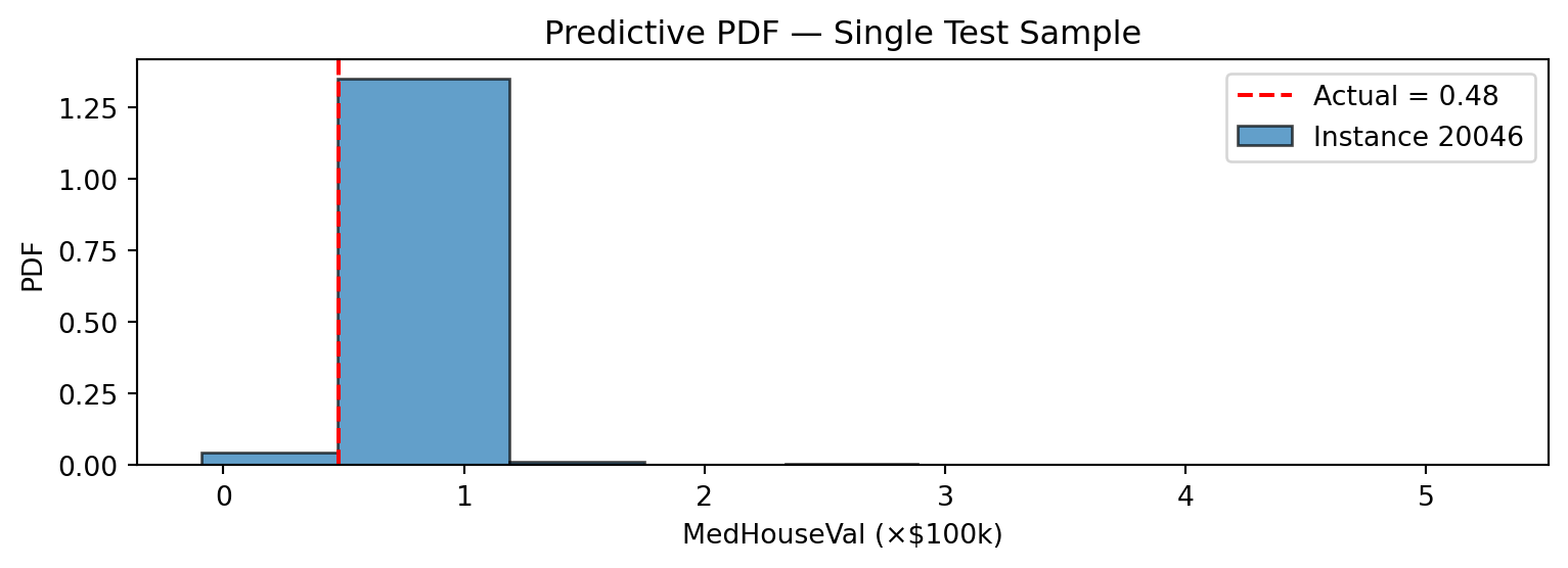

# Four samples side by side
fig, axes = plt.subplots(1, 4, figsize=(16, 3))
for ax, i in zip(axes, range(4)):
    row_idx = y_test.index[i]
    dist.loc[[row_idx]].plot(ax=ax, alpha=0.7)
    ax.axvline(y_test.iloc[i], color="red", linestyle="--", linewidth=1.5)
    ax.set_title(f"Sample {i}")
    ax.set_xlabel("y")

plt.suptitle("Predictive PDFs — PartitionTreeRegressor", y=1.02)
plt.tight_layout()
plt.show()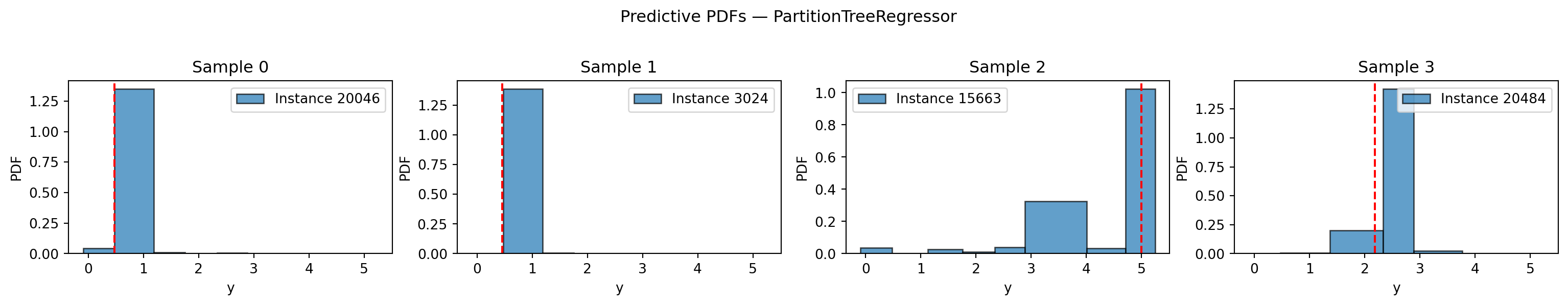

6. Partition Forest — Better Calibrated Distributions

PartitionForestRegressor averages the conditional densities from multiple trees, producing smoother and better-calibrated distributions.

from partition_tree.skpro import PartitionForestRegressor

pf = PartitionForestRegressor(
    n_estimators=50,
    random_state=42,
    min_volume_fraction=0.1,
    output_distribution="mixture",
)
pf.fit(X_train, y_train)

dist_forest = pf.predict_proba(X_test)
y_pred_forest = pf.predict(X_test)

7. Random Forest comparison

from sklearn.ensemble import RandomForestRegressor

rf = RandomForestRegressor(
    n_estimators=50,
    random_state=42,
)
rf.fit(X_train, y_train)
y_pred_rf = rf.predict(X_test)

Point metrics comparison

pd.DataFrame({
    "Model": ["DecisionTree (CART)", "PartitionTree", "PartitionForest", "RandomForest"],
    "RMSE": [
        root_mean_squared_error(y_test, y_pred_cart),
        root_mean_squared_error(y_test, y_pred_pt),
        root_mean_squared_error(y_test, y_pred_forest),
        root_mean_squared_error(y_test, y_pred_rf),
    ],
    "R²": [
        r2_score(y_test, y_pred_cart),
        r2_score(y_test, y_pred_pt),
        r2_score(y_test, y_pred_forest),
        r2_score(y_test, y_pred_rf),
    ],
}).round(4)

	Model	RMSE	R²
0	DecisionTree (CART)	0.7037	0.6221
1	PartitionTree	0.5879	0.7362
2	PartitionForest	0.5076	0.8034
3	RandomForest	0.5072	0.8037

Coverage comparison

lower_f = dist_forest.ppf(0.10)["MedHouseVal"]
upper_f = dist_forest.ppf(0.90)["MedHouseVal"]
covered_f = ((y_true >= lower_f.values) & (y_true <= upper_f.values)).mean()

print(f"Tree   80% PI coverage: {covered:.1%}")
print(f"Forest 80% PI coverage: {covered_f:.1%}")

Tree   80% PI coverage: 76.1%
Forest 80% PI coverage: 94.1%

`output_distribution` option

PartitionForestRegressor supports two strategies for combining per-tree distributions:

`output_distribution`	Description
`"merged"` (default)	Merges all tree breakpoints into one `IntervalDistribution`. Full API support, computed once at predict time.
`"mixture"`	Returns a `MixtureIntervalDistribution`. PDF/CDF/quantiles computed on-the-fly; avoids the merge cost.

pf_mix = PartitionForestRegressor(
    n_estimators=50,
    random_state=42,
    min_volume_fraction=0.1,
    output_distribution="mixture",
)
pf_mix.fit(X_train, y_train)
dist_mix = pf_mix.predict_proba(X_test)

8. Feature Importances

Feature importances are accumulated log-loss gain across all splits:

importances = pt.get_feature_importances(normalize=True)
for feat, imp in importances.items():
    print(f"  {feat:>20s}: {imp:.4f}")

    target_MedHouseVal: 0.2436
                MedInc: 0.1911
             Longitude: 0.1513
              Latitude: 0.1367
              AveOccup: 0.1089
              AveRooms: 0.0481
              HouseAge: 0.0434
            Population: 0.0411
             AveBedrms: 0.0358

Setup

1. Baseline — Decision Tree (CART)

2. Single Partition Tree

Fit and point prediction

Comparison with CART

Probabilistic prediction

3. The IntervalDistribution API

4. Prediction Intervals

5. Visualizing the Predictive PDF

6. Partition Forest — Better Calibrated Distributions

7. Random Forest comparison

Point metrics comparison

Coverage comparison

output_distribution option

8. Feature Importances

3. The `IntervalDistribution` API

`output_distribution` option