Quantized Target with partition_tree.skpro

This notebook shows how to use the skpro PartitionTreeRegressor when the target lives on a fixed lattice, such as values rounded to the nearest 0.25.

The key step is passing a quantized target override through dtype_overrides with Domain.quantized_continuous(resolution).

import matplotlib.pyplot as plt
import numpy as np
import pandas as pd
from sklearn.metrics import mean_absolute_error
from sklearn.model_selection import train_test_split

from partition_tree import Domain
from partition_tree.skpro import PartitionTreeRegressor

rng = np.random.default_rng(42)
resolution = 0.25
n_samples = 500

x1 = rng.uniform(-3.0, 3.0, size=n_samples)
x2 = rng.normal(loc=0.0, scale=1.0, size=n_samples)
signal = 3.0 + 1.8 * np.sin(x1) + 0.7 * x2
noise = rng.normal(scale=0.20, size=n_samples)
y_raw = signal + noise
y_quantized = np.round(y_raw / resolution) * resolution

X = pd.DataFrame({"x1": x1, "x2": x2})
y = pd.DataFrame({"target": y_quantized})

alignment_error = np.abs((y["target"] / resolution) - np.round(y["target"] / resolution)).max()
print(f"max alignment error: {alignment_error:.2e}")
print(y.head())

X_train, X_test, y_train, y_test = train_test_split(
    X, y, test_size=0.25, random_state=42
)

max alignment error: 0.00e+00
   target
0    5.50
1    2.50
2    5.00
3    4.75
4    1.75

Fit a probabilistic tree with a quantized target

For a single-target skpro regression problem, the wrapper keeps the target column name as target, so the override key must use that same name.

model = PartitionTreeRegressor(
    max_leaves=4000,
    max_depth=600,
    min_samples_xy=0,
    min_samples_x=50,
    min_samples_y=0,
    min_samples_split=1,
    min_volume_fraction=0,
    random_state=42,
    dtype_overrides={"target": Domain.quantized_continuous(resolution)},
)
model.fit(X_train, y_train)

root_partitions = model.partition_tree_.get_nodes_info()[0]["partitions"]
root_partitions["target"]

{'type': 'quantized_continuous',
 'low': -1.875,
 'high': 7.125,
 'resolution': 0.25,
 'lower_closed': True,
 'upper_closed': True}

dist = model.predict_proba(X_test)
mean_pred = model.predict(X_test)["target"]
lower_80 = dist.ppf(0.10)["target"]
upper_80 = dist.ppf(0.90)["target"]

summary = pd.DataFrame({
    "y_true": y_test["target"],
    "mean": mean_pred,
    "p10": lower_80,
    "p90": upper_80,
}).head(10)
summary

	y_true	mean	p10	p90
361	3.00	3.713110	2.315500	5.842628
73	0.75	1.541523	1.169308	1.871176
374	1.50	1.711535	1.208367	2.521245
155	4.50	4.022503	3.400502	4.746518
104	6.00	4.319656	2.467867	5.655662
394	1.25	1.133886	0.312259	2.187634
377	1.00	1.588658	0.398932	2.964457
124	2.75	1.856689	1.409734	2.353638
68	3.00	1.856689	1.409734	2.353638
450	2.50	1.856689	1.409734	2.353638

coverage_80 = ((y_test["target"] >= lower_80) & (y_test["target"] <= upper_80)).mean()
mae = mean_absolute_error(y_test["target"], mean_pred)

print(f"MAE: {mae:.3f}")
print(f"80% prediction interval coverage: {coverage_80:.1%}")

MAE: 0.539
80% prediction interval coverage: 74.4%

rows = list(X_test.index[:3])
fig, axes = plt.subplots(1, 3, figsize=(15, 3.5), sharey=True)

for ax, row_idx in zip(axes, rows):
    dist_single = dist.loc[row_idx]
    dist_single.plot(ax=ax, alpha=0.7)
    ax.axvline(y_test.loc[row_idx, "target"], color="crimson", linestyle="--", linewidth=2)
    ax.set_title(f"sample {row_idx}")
    ax.set_xlabel("target")

axes[0].set_ylabel("density")
fig.suptitle("Predictive distributions for a quantized target", y=1.03)
plt.tight_layout()
plt.show()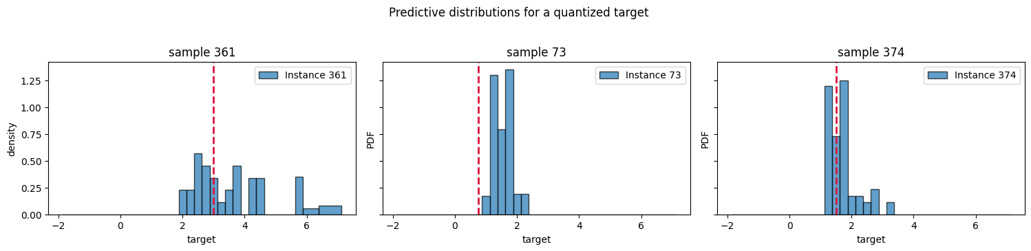

dist_single.loc[73]

IntervalDistribution(columns=Index(['target'], dtype='object'),
                     index=Index([374], dtype='int64'),
                     intervals=[[(-1.875, 0.625), (0.625, 2.375),
                                 (2.375, 5.375), (5.375, 7.125)]],
                     pdf_values=[array([0.00144872, 0.52783759, 0.02301354, 0.0020696 ])])

Please rerun this cell to show the HTML repr or trust the notebook.

y_test.sort_values("target")

	target
262	-0.00
15	0.00
408	0.25
148	0.25
172	0.25
...	...
433	5.50
356	6.00
290	6.00
104	6.00
72	6.50

125 rows × 1 columns